Classifying Obama/McCain Voters Using A Decision Tree

What data are going to use?

The synthetic dataset contains information about voting preferences of a number of voters in 2008 US Presidential Elections together with some demographic information available for the voters.

The data set consists of the following attributes:

Id. Unique Id of each row of a file.
Party. Political party affiliation of the voter.
1 Democratic
2 Republican
3 Independent

Ideology. Political ideology of the voter.
1 Liberal
2 Moderate
3 Conservative

Race. Race of the voter.
1 Black (African-American)
2 White (Caucasian)
3 Other

Gender. Gender of the voter.
1 Male
2 Female

Religion. Religion of the voter.
1 Protestant
2 Catholic
3 Other

Income. The income bracket (annual income) of the voter's family.
1 Less than $30,000
2 $30,000 - $49,999
3 $50,000 - $74,999
4 $75,000 - $99,999
5 $100,000 - $149,999
6 Over $150,000

Education. The highest level of education for the voter.
1 High school diploma or less
2 Undergraduate study/degree
3 Postgraduate study/degree

Age. The age group of the voter.
1 18 - 29
2 30 - 44
3 45 - 64
4 65 and over

Region. The geographic region where the voter lives.
1 Northeast ME, NH, VT, MA, RI, CT, PA, NY, NJ, DE, MD, DC
2 South(east) VA, WV, KY, NC, SC, TN, GA, FL, AL, MS, LA, AR, TX, OK
3 Midwest OH, IN, MI, IL, MO, IA, MN, WI, ND, SD, NE, KS
4 West MT, ID, WA, AK, HI, WY, CO, UT, OR, NV, AZ, NM, CA

BushApproval. Indicator whether the voter approves of George W. Bush in his capacity as the President of the US.
1 Approve'
2 Disapprove

Goal

Determine who voters will vote using demographic data.

RCode

	> library(pacman)
	> pacman::p_load(tree, caret)
	> data <- read.csv(file.choose())
	> str(data)
	'data.frame': 1000 obs. of 12 variables:
	$ Id : int 1 2 3 4 5 6 7 8 9 10 ...
	$ Political.Party: Factor w/ 3 levels "Democratic","Independent",..: 1 1 2 1 3 2 3 2 3 1 ...
	$ Ideology : Factor w/ 3 levels "Conservative",..: 2 2 3 3 1 1 1 2 3 3 ...
	$ Race : Factor w/ 3 levels "Black","Other",..: 3 1 3 3 3 3 3 3 1 3 ...
	$ Gender : Factor w/ 2 levels "Female","Male": 1 1 1 1 1 2 1 2 2 1 ...
	$ Religion : Factor w/ 3 levels "Catholic","Other",..: 1 3 1 3 3 3 3 1 3 1 ...
	$ Family.Income : Factor w/ 6 levels "100000-149999",..: 4 2 1 3 1 2 4 1 2 1 ...
	$ Education : Factor w/ 3 levels "College","H.S. diploma or less",..: 1 2 3 3 2 1 1 1 1 1 ...
	$ Age : Factor w/ 4 levels "18-29","30-44",..: 3 3 3 3 4 3 2 1 2 3 ...
	$ Region : Factor w/ 4 levels "Midwest","Northeast",..: 1 2 2 2 2 2 1 2 1 1 ...
	$ Bush.Approval : Factor w/ 2 levels "Approve","Disapprove": 1 2 2 2 2 2 2 1 2 2 ...
	$ Vote : Factor w/ 2 levels "McCain","Obama": 2 2 2 2 1 2 2 2 2 2 ...
	> names(data)
	[1] "Id" "Political.Party" "Ideology" "Race" "Gender"
	[6] "Religion" "Family.Income" "Education" "Age" "Region"
	[11] "Bush.Approval" "Vote"
	> newdata <- data[, c(2:12)]
	> names(newdata)
	[1] "Political.Party" "Ideology" "Race" "Gender" "Religion"
	[6] "Family.Income" "Education" "Age" "Region" "Bush.Approval"
	[11] "Vote"
	> initialtree <- tree(Vote ~ ., newdata)
	> summary(initialtree)
	Classification tree:
	tree(formula = Vote ~ ., data = newdata)
	Variables actually used in tree construction:
	[1] "Age" "Family.Income" "Political.Party" "Race" "Bush.Approval"
	[6] "Ideology" "Region"
	Number of terminal nodes: 20
	Residual mean deviance: 0.06371 = 62.44 / 980
	Misclassification error rate: 0.016 = 16 / 1000
	> plot(initialtree)
	> text(initialtree, pretty = 2)
	> title(main = "Initial Tree")

view raw Election Tree 1.r hosted with ❤ by GitHub

	> #Split
	> set.seed(1)
	> trainIndex <- sample(nrow(newdata), nrow(newdata) * .6)
	> train <- newdata[trainIndex, ]
	> test <- newdata[-trainIndex, ]
	> tree <- tree(Vote ~ ., data = test)
	> plot(tree)
	> text(tree, pretty = 2)
	> title(main = "Train Tree")
	> summary(tree)
	Classification tree:
	tree(formula = Vote ~ ., data = test)
	Variables actually used in tree construction:
	[1] "Age" "Family.Income" "Political.Party" "Bush.Approval" "Ideology"
	[6] "Race" "Region"
	Number of terminal nodes: 12
	Residual mean deviance: 0.1024 = 39.74 / 388
	Misclassification error rate: 0.0275 = 11 / 400

view raw Election Tree 2.r hosted with ❤ by GitHub

	> set.seed(2)
	> cvtest <- cv.tree(tree, FUN = prune.misclass)
	> names(cvtest)
	[1] "size" "dev" "k" "method"
	> cvtest
	$size
	[1] 12 8 6 4 1
	$dev
	[1] 22 22 25 28 28
	$k
	[1] -Inf 0.000000 1.000000 2.500000 2.666667
	$method
	[1] "misclass"
	attr(,"class")
	[1] "prune" "tree.sequence"
	> par(mfrow = c(1, 3))
	> plot(cvtest$size, cvtest$dev, type = "b")
	> plot(cvtest$k, cvtest$dev, type = "b")
	> plot(cvtest)
	> prune <- prune.misclass(tree, best = 8)
	> par(mfrow = c(1, 1))
	> plot(prune)
	> text(prune, pretty = 0)
	> title(main = "Pruned Tree")

view raw Election Tree 3.r hosted with ❤ by GitHub

	> predictclass <- predict(prune, test, type = "class")
	> predicttree <- predict(prune, test)
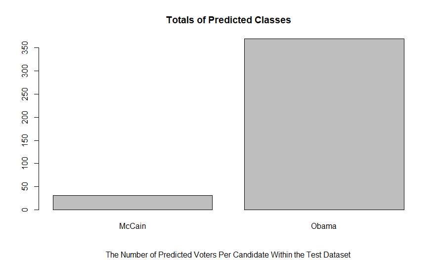
	> confusionMatrix(predictclass, test$Vote)
	Confusion Matrix and Statistics
	Reference
	Prediction McCain Obama
	McCain 23 8
	Obama 3 366
	Accuracy : 0.9725
	95% CI : (0.9513, 0.9862)
	No Information Rate : 0.935
	P-Value [Acc > NIR] : 0.0005747
	Kappa : 0.7923
	Mcnemar's Test P-Value : 0.2278000
	Sensitivity : 0.8846
	Specificity : 0.9786
	Pos Pred Value : 0.7419
	Neg Pred Value : 0.9919
	Prevalence : 0.0650
	Detection Rate : 0.0575
	Detection Prevalence : 0.0775
	Balanced Accuracy : 0.9316
	'Positive' Class : McCain
	>plot(predictclass, main = "Totals of Predicted Classes", sub= "The Number of Predicted Voters Per Candidate Within the Test Dataset")
	> head(predictclass)
	[1] Obama Obama Obama Obama Obama Obama
	Levels: McCain Obama
	> head(predicttree)
	McCain Obama
	3 0.04166667 0.9583333
	6 0.04166667 0.9583333
	8 0.00000000 1.0000000
	9 0.00000000 1.0000000
	10 0.04166667 0.9583333
	11 0.00000000 1.0000000

view raw Election Tree 4.r hosted with ❤ by GitHub