A client wants to launch an ad campaign. He has already made a similar campaign in the past and now wants to leverage historical data to assess the impact of his ads before making new investments.
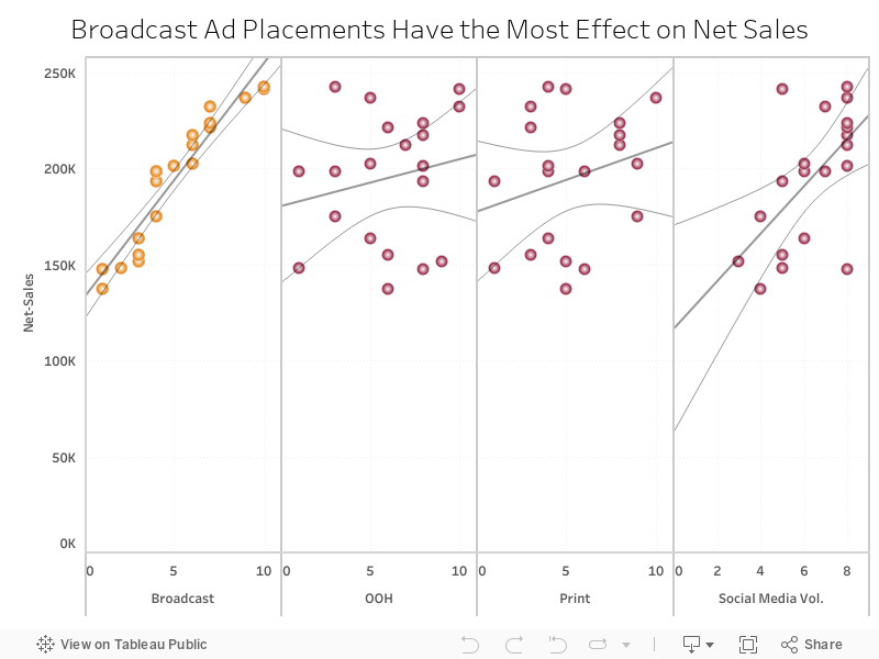
I already ran a regression analysis on Tableau and found that broadcast has the most impact on net sales.
Coeff:
(Intercept) - 133108.8
Broadcast - 12141.9
P-value - 1.95e-10
Adj. R Sqaured - 0.8944
But let's try it using R.
What data are going to use?
A spreadsheet with 21 rows and the ff. columns for our purpose:- Broadcast - number of placements in broadcast media
- Out-of-Home - number of out-of-home ads
- Print - number of ads in print
- Net.Sales - net of sales
Here's how it looks:
Short Answer:
Coeff:
But let's try it using R.
R Code:
This file contains bidirectional Unicode text that may be interpreted or compiled differently than what appears below. To review, open the file in an editor that reveals hidden Unicode characters.
Learn more about bidirectional Unicode characters
> broadsales <- read.csv(file.choose()) | |
> head(broadsales) | |
DATE GEO OUT.OF.HOME PRINT BROADCAST NET.SALES UNIQUE.WEBSITE.VISITORS SOCIAL.MEDIA.VOLUM SALES.INCREASE | |
1 2/13/17 Kentucky 6 5 1 137452 3974 4 -3 | |
2 2/12/17 NI 8 6 1 147376 3732 8 7 | |
3 3/7/17 Virginia 1 1 2 148252 3127 5 2 | |
4 3/14/17 SIC 9 5 3 151842 3091 3 7 | |
5 2/5/17 DE 6 3 3 155207 4791 5 8 | |
6 1/3/17 IN 5 4 3 163855 5066 6 5 | |
U.W.VISITORS.INCREASE SOCIAL.MEDIA.VOLUME.INCREASE | |
1 -2 0 | |
2 -3 7 | |
3 0 -3 | |
4 2 5 | |
5 7 -2 | |
6 -3 0 | |
> attach(broadsales) | |
fit <- lm(NET.SALES~OUT.OF.HOME+PRINT+BROADCAST) | |
> summary(fit) | |
Call: | |
lm(formula = NET.SALES ~ OUT.OF.HOME + PRINT + BROADCAST) | |
Residuals: | |
Min 1Q Median 3Q Max | |
-18114.1 -8083.5 -712.5 8061.8 17124.8 | |
Coefficients: | |
Estimate Std. Error t value Pr(>|t|) | |
(Intercept) 132643.92 8859.37 14.972 7.86e-11 *** | |
OUT.OF.HOME 126.76 1015.82 0.125 0.902 | |
PRINT -42.76 1072.75 -0.040 0.969 | |
BROADCAST 12128.39 1070.40 11.331 4.70e-09 *** | |
--- | |
Signif. codes: 0 ‘***’ 0.001 ‘**’ 0.01 ‘*’ 0.05 ‘.’ 0.1 ‘ ’ 1 | |
Residual standard error: 11870 on 16 degrees of freedom | |
Multiple R-squared: 0.9001, Adjusted R-squared: 0.8813 | |
F-statistic: 48.04 on 3 and 16 DF, p-value: 3.169e-08 | |
#BROADCAST is the only channel with a low P-value | |
> plot(BROADCAST, NET.SALES) | |
> abline(NET.SALES~BROADCAST) |
Comments
Post a Comment